gpu-deployment-tutorial
Monitoring and Debugging GPU Python Workloads
Moving a Python workload onto a GPU doesn’t automatically make the full workflow faster in every scenario. The GPU can execute parallel work very quickly, but the workflow still has overheads for cold starts, data movement, Python overhead, synchronization, and any CPU-only stages left in the path. If your GPU code runs but doesn’t get the speedup you expected, or if the GPU looks idle while the program is busy, the cause is almost always one of those costs rather than the GPU itself.
This section gives you the tools to diagnose those overheads and fix them. We’ll use terminal monitoring tools, Python profilers, and GPU timeline traces to answer one question: which part of this workflow is the limiter, and how do we make it faster?
To keep it concrete, we’ll follow a single workload from start to finish. We’ll take a year of global temperature data, run a standard analysis on it, port that analysis to the GPU, watch it underperform, and use each tool in turn to find and fix the bottleneck. Every tool we introduce answers a question the previous one couldn’t.
Before we run Python code
Start where every GPU debugging session should start: the VM.
nvidia-smi
On a working VM you should see a table with the GPU name, driver version, the CUDA version reported by the driver, memory usage, utilization, and a process table. On a Brev VM with an L4 it looks something like this:
$ nvidia-smi
+-----------------------------------------------------------------------------------------+
| NVIDIA-SMI 580.159.03             Driver Version: 580.159.03     CUDA Version: 13.0     |
+-----------------------------------------+------------------------+----------------------+
| GPU  Name                 Persistence-M | Bus-Id          Disp.A | Volatile Uncorr. ECC |
| Fan  Temp   Perf          Pwr:Usage/Cap |           Memory-Usage | GPU-Util  Compute M. |
|                                         |                        |               MIG M. |
|=========================================+========================+======================|
|   0  NVIDIA L4                      On  |   00000000:00:03.0 Off |                    0 |
| N/A   40C    P8             13W /   72W |       0MiB /  23034MiB |      0%      Default |
|                                         |                        |                  N/A |
+-----------------------------------------+------------------------+----------------------+

+-----------------------------------------------------------------------------------------+
| Processes:                                                                              |
|  GPU   GI   CI              PID   Type   Process name                        GPU Memory |
|        ID   ID                                                               Usage      |
|=========================================================================================|
|  No running processes found                                                             |
+-----------------------------------------------------------------------------------------
For a shorter listing of GPUs:
nvidia-smi -L
For a detailed dump suitable for a support report:
nvidia-smi -q
How should we read this? If nvidia-smi successfully prints that information it confirms that the host driver can see the GPU, and it reports the driver version and the CUDA compatibility level. It does not confirm that your Python environment is healthy. That distinction matters because the host can have a working driver while your active Python environment is missing CUDA runtime libraries or contains incompatible packages.
If nvidia-smi fails, stop. Don’t debug the Python environment yet. Fix the VM, driver, or container/runtime layer first.
Install the terminal monitoring tools
nvidia-smi is a good first sanity check, but it’s coarse. For live monitoring, install nvtop:
sudo apt update
sudo apt install -y nvtop
Start it:
nvtop
Press q to quit.
You can also poll nvidia-smi on a tight interval:
watch -n 1 nvidia-smi
You can exit of this view with Ctrl+C.
Reach for watch nvidia-smi when you want to see snapshots of the current GPU state. Use nvtop when you want to see a timeline to check whether a running process is keeping the GPU busy.
For fine-grained timeline profiling, install Nsight Systems. This tool is great for it when the GPU looks busy but the workload is still slow: it lays out CPU/GPU memory transfers, CUDA API calls, kernel launches, and synchronization points on a single timeline. We install it now and use it in detail later in this section. On a fresh VM you first need the NVIDIA CUDA apt repository, since the Nsight Systems package lives there:
wget https://developer.download.nvidia.com/compute/cuda/repos/ubuntu2204/x86_64/cuda-keyring_1.1-1_all.deb
sudo dpkg -i cuda-keyring_1.1-1_all.deb
sudo apt update
Then install Nsight Systems:
sudo apt install -y cuda-nsight-systems-13-0
Confirm nsys is on PATH:
which nsys
nsys --version
nsys status --environment
If nsys isn’t found, refuses to run, or warns that sampling is restricted, see Troubleshooting Nsight Systems at the end of this section before continuing.
Check the Python environment
The rest of this section works through an xarray + CuPy example on real climate data, so the environment needs those libraries (xarray, netCDF4, CuPy, and cupy-xarray) in addition to the profilers.
Use the Python environment you created earlier in the tutorial. The exact package manager doesn’t matter. What matters is that python points to the environment you need. Activate it first. On Brev, the uv path installed into the system venv at ~/.venv:
source ~/.venv/bin/activate
(If you used conda, run conda activate tutorial-env instead and if you used pixi, use pixi shell --manifest-path envs/pixi.toml)
Then confirm python points where you expect:
which python
python --version
Verify that you have all the packages needed for this section:
python - <<'PY'
import numpy
import cupy
import pandas
import xarray
import cupy_xarray  # noqa: F401  # registers the .cupy accessor on xarray objects
import cuda.core.system as system

print("numpy", numpy.__version__)
print("cupy", cupy.__version__)
print("pandas", pandas.__version__)
print("xarray", xarray.__version__)
print("cuda device count", system.get_num_devices())
PY
If this block fails, fix the environment before proceeding. For example, if CuPy fails with a message about libnvrtc.so.13, that’s CuPy trying to load the NVIDIA Runtime Compiler library and not finding it. You’ll need to reinstall the CUDA toolkit or update the CuPy bindings before CuPy can use the GPU.
A Python view of the GPU with cuda.core
We’ll use cuda.core as the Python-side probe. This isn’t a replacement for nvidia-smi. It answers a different question.
nvidia-smi answers: does the host driver see the GPU?
cuda.core answers: can this Python environment load the CUDA libraries it needs to talk to the driver?
The scripts/gpu-probe-cuda-core.py script asks CUDA how many devices it can see, then prints each device’s name, compute capability, and memory. Run it:
python scripts/gpu-probe-cuda-core.py
If both nvidia-smi and this script succeed, the host and the active Python runtime both see the GPU. If nvidia-smi succeeds but this script fails, the host is fine but the Python environment is not. That’s an environment issue, not a hardware issue, and it’s worth catching now before we start using the GPU.
Profilers we’ll use
We already have nvidia-smi, nvtop, and cuda.core. Three more tools fill out the kit, and it’s worth knowing what each one answers before we reach for it.
cProfile is Python’s built-in CPU-side function profiler. It answers: which Python functions ran, how many times, and how much cumulative time did they consume? It’s the right tool when the GPU looks idle, because Python preprocessing, parsing, or object construction can be a bottleneck before any GPU work begins.
SnakeViz is a visual viewer for cProfile output. It doesn’t collect any new data, but renders the .prof file in a browser so the dominant functions are easy to see.
Nsight Systems is a system timeline profiler. The command-line tool is nsys. For Python GPU workloads it answers a different question from cProfile: what happened across the CPU threads, CUDA API calls, memory copies, synchronization points, and GPU kernels over time. It’s especially good at spotting CPU/GPU transfers, gaps between kernels, many tiny launches, and synchronization points that force Python to wait. We use nsys profile to produce .nsys-rep files, which open in the Nsight Systems UI for inspection.
Which tool to use first depends on the symptom:
| Symptom | First tool | Why |
|---|---|---|
| Host may not see the GPU | nvidia-smi |
Confirms driver-level GPU visibility. |
| Python may not see CUDA devices | cuda.core |
Confirms the active Python runtime can inspect CUDA devices. |
| GPU may be idle during a run | nvtop or watch nvidia-smi |
Shows live utilization and process memory. |
| Python preprocessing may dominate | cProfile and SnakeViz |
Shows CPU-side function time. |
| Transfers, launch gaps, or synchronization may dominate | nsys |
Shows CPU/GPU timeline behavior. |
With the tools mapped, let’s understand a couple of GPU concepts.
Timing GPU work correctly
Both the host and our Python environment can see the GPU. Before we put a real workload on it, we need to understand a couple of concepts: how to time GPU work honestly, and why moving data is expensive.
GPU work is often asynchronous. Python can enqueue work and keep executing before the GPU has finished. To see this, open the python interpreter and run the following example:
import time
import cupy as cp

# Warmup
cp.arange(100_000_000, dtype=cp.float32) * 2
cp.cuda.Stream.null.synchronize()

start = time.perf_counter()
result = cp.arange(100_000_000, dtype=cp.float32) * 2
t_cpu = time.perf_counter() - start       # CPU stopped here, GPU still running

cp.cuda.Stream.null.synchronize()
t_gpu = time.perf_counter() - start       # GPU actually finished here

print(f"without sync: {t_cpu * 1e3:.3f} ms  ← wrong")
print(f"with sync:    {t_gpu * 1e3:.3f} ms  ← correct")
Even with synchronize(), treat these timings as good estimates, not production benchmarks. They’re accurate enough to compare how long the GPU spent on a task, which is all we need here.
Why data transfer becomes a bottleneck
The CPU and GPU have separate memory. A NumPy array lives in host memory. A CuPy array lives in device memory. Moving data from host to device is a CPU-to-GPU transfer, and moving it back is a GPU-to-CPU transfer.
Those transfers aren’t free. For a small workload, the transfer overhead can outweigh the benefit of GPU computation. For a larger workflow, repeated transfers can erase an otherwise good speedup. This is why just using the GPU isn’t enough. The useful question is whether enough of the expensive work stayed on the GPU long enough to justify the transfer.
Some rules of thumb to use:
- Transfer once when you can.
- Do enough GPU work to pay for the transfer.
- Keep the hot path on the GPU.
- Reduce, aggregate, or sample before moving data back to the CPU.
- Avoid unnecessary round trips between CPU and GPU.
The examples below are variations on this idea. The naive GPU port we’re about to write moves the matrix back to the CPU before the expensive step. The same mistake shows up in visualization, when someone pulls a full GPU array back to the host just to plot a small sample. The fix is symmetric: sample, aggregate, or filter on the GPU first, and transfer only the small result. The same logic applies to any “give me a peek at the data” operation, whether it feeds a plot, an inspection, or a downstream CPU library.
Now lets work through a real workload on a dataset and understand what’s happening under the surface
Get the dataset
Every example below uses the same NCEP/NCAR Reanalysis surface temperature file: 4x daily air temperature for 2025 on a 2.5 degree global grid. Download it once into your working directory:
wget "https://downloads.psl.noaa.gov/Datasets/ncep.reanalysis/surface/air.sig995.2025.nc"
The file is about 22 MB on disk. Confirm xarray can open it and that the array has the expected shape:
python - <<'PY'
import xarray as xr

ds = xr.open_dataset("air.sig995.2025.nc")
air = ds["air"]
print("variable:", air.name)
print("dims:", air.dims)
print("shape:", air.shape)
print("dtype:", air.dtype)
print("size MiB:", round(air.nbytes / 1024**2, 1))
PY
The output should look like:
variable: air
dims: ('time', 'lat', 'lon')
shape: (1460, 73, 144)
dtype: float32
size MiB: 58.6
The on-disk file is compressed, so the in-memory array (about 58.6 MiB once xarray unpacks it to float32) is larger than the 22 MB you downloaded. That’s the dataset every example in this section builds on.
Establishing a CPU baseline
We start on the CPU. The script loads the temperature dataset, reshapes it to a time-by-space matrix, subtracts the time mean at each grid point to get anomalies, then runs an SVD to find the dominant spatial pattern. The SVD is the expensive step. This is the recipe for an Empirical Orthogonal Function (EOF) analysis, which is the principal component analysis applied to gridded climate data.
That analysis lives in scripts/xarray-cpu-baseline.py. Run it:
python scripts/xarray-cpu-baseline.py
Then profile it to see where the time actually goes:
python -m cProfile -o profile-xarray-cpu.prof scripts/xarray-cpu-baseline.py
python -m snakeviz -s profile-xarray-cpu.prof
SnakeViz starts a local web server (by default at http://127.0.0.1:8080). On a remote Brev VM that port isn’t reachable from your laptop until you forward it. From your laptop, forward the port, then open the printed URL in your local browser:
brev port-forward <your-instance-name> -p 8080:8080
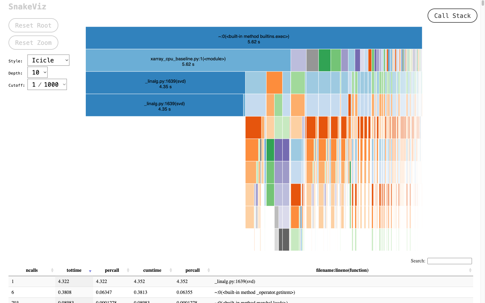
The largest block in the SnakeViz icicle chart should be the svd call (labeled _linalg.py:...(svd)), taking the large majority of the runtime. cProfile pools the time there. The reshape and mean-subtraction blocks are visibly smaller. If they weren’t, a GPU port wouldn’t have anything worth speeding up.
We now have a baseline number and a profile that says the SVD is the computationally expensive operation. That’s our target. When we build a GPU version, this is the number we compare against, and “the SVD” is the part we want to accelerate.
A naive GPU port that moves back to CPU
Here’s a tempting mistake. We move the data to the GPU, do the preprocessing on the GPU, then move the matrix back to the CPU before the expensive SVD. This uses the GPU, but not for the operation that matters most.
The naive port lives in scripts/xarray-cupy-naive.py.
Compared with the CPU baseline, this port moves the field onto the GPU for the reshape and mean-subtraction, then copies it back to the CPU before the SVD, so the expensive step still runs on the CPU:
+import cupy as cp
 import numpy as np
 import xarray as xr

-T = air.to_numpy()
+T = cp.asarray(air)

 X = X - X.mean(axis=0, keepdims=True)
+X = X.get()
 U, S, Vt = np.linalg.svd(X, full_matrices=False)
Exercise: before running it, predict the timing. This script does the data load, reshape, and mean-subtraction on the GPU, then runs the SVD. Will it beat the CPU baseline? Run it, then profile it the same way you profiled the baseline (
python -m cProfile -o profile-xarray-cupy-naive.prof scripts/xarray-cupy-naive.py, thenpython -m snakeviz -s profile-xarray-cupy-naive.prof) and see which call still dominates the runtime.
The mistake lives in these two lines:
X = X.get()
U, S, Vt = np.linalg.svd(X, full_matrices=False)
We did the computationally inexpensive part on the GPU and the expensive part on the CPU. Run it, and watch the GPU while it runs. In one terminal:
python scripts/xarray-cupy-naive.py
In a second terminal:
nvtop
This is the moment nvtop is the right tool. You’ll see the GPU light up briefly while the data transfers over and the reshape and mean-subtraction run, then drop back to idle and sit there while the CPU grinds through the SVD. Seeing the GPU go idle in the middle of a run that’s supposed to be “GPU accelerated” is the problem.
Going deeper with Nsight Systems
nvtop told us that the GPU went idle. To see exactly what happened, and in what order, we reach for another tool and capture a timeline:
nsys profile \
  --trace cuda,osrt \
  --cuda-memory-usage true \
  --force-overwrite true \
  --output profile-xarray-cupy-naive \
  $(which python) scripts/xarray-cupy-naive.py
These are what the various flags are for (For more information, check the Nsight User Guide):
--trace cuda,osrt: record GPU/CUDA activity plus CPU-side OS-runtime waits.--cuda-memory-usage true: track GPU memory allocation over the run.--force-overwrite true: replace an existing report of the same name.--output profile-xarray-cupy-naive: name of the.nsys-repfile.$(which python) scripts/xarray-cupy-naive.py: the program to profile
At the end of the run, nsys prints where it wrote the report. On Brev that’s your home directory:
Generated:
    /home/ubuntu/profile-xarray-cupy-naive.nsys-rep
Capturing happens on the VM, but exploring the timeline needs the Nsight Systems desktop app, which runs on your laptop, not the VM. So you pull the report down and open it locally.
Install the Nsight Systems GUI on your laptop once, from the Nsight Systems page. This desktop application is separate from the nsys command-line tool you installed on the VM.
Then copy the report down from Brev. Run this from a new terminal on your laptop (not the VM) in the location you want the file to be saved:
brev copy <your-instance-name>:~/profile-xarray-cupy-naive.nsys-rep .
brev copy takes <source> <destination>, so a <instance>:<remote-path> source and a local . destination pulls the .nsys-rep into your current directory. If ~ doesn’t resolve on the remote, use the absolute path /home/ubuntu/profile-xarray-cupy-naive.nsys-rep.
Finally, open it: launch Nsight Systems and use File > Open to select the .nsys-rep (or run nsys-ui profile-xarray-cupy-naive.nsys-rep from a terminal if the GUI’s launcher is on your PATH). Zoom into the CUDA HW rows to explore the timeline.
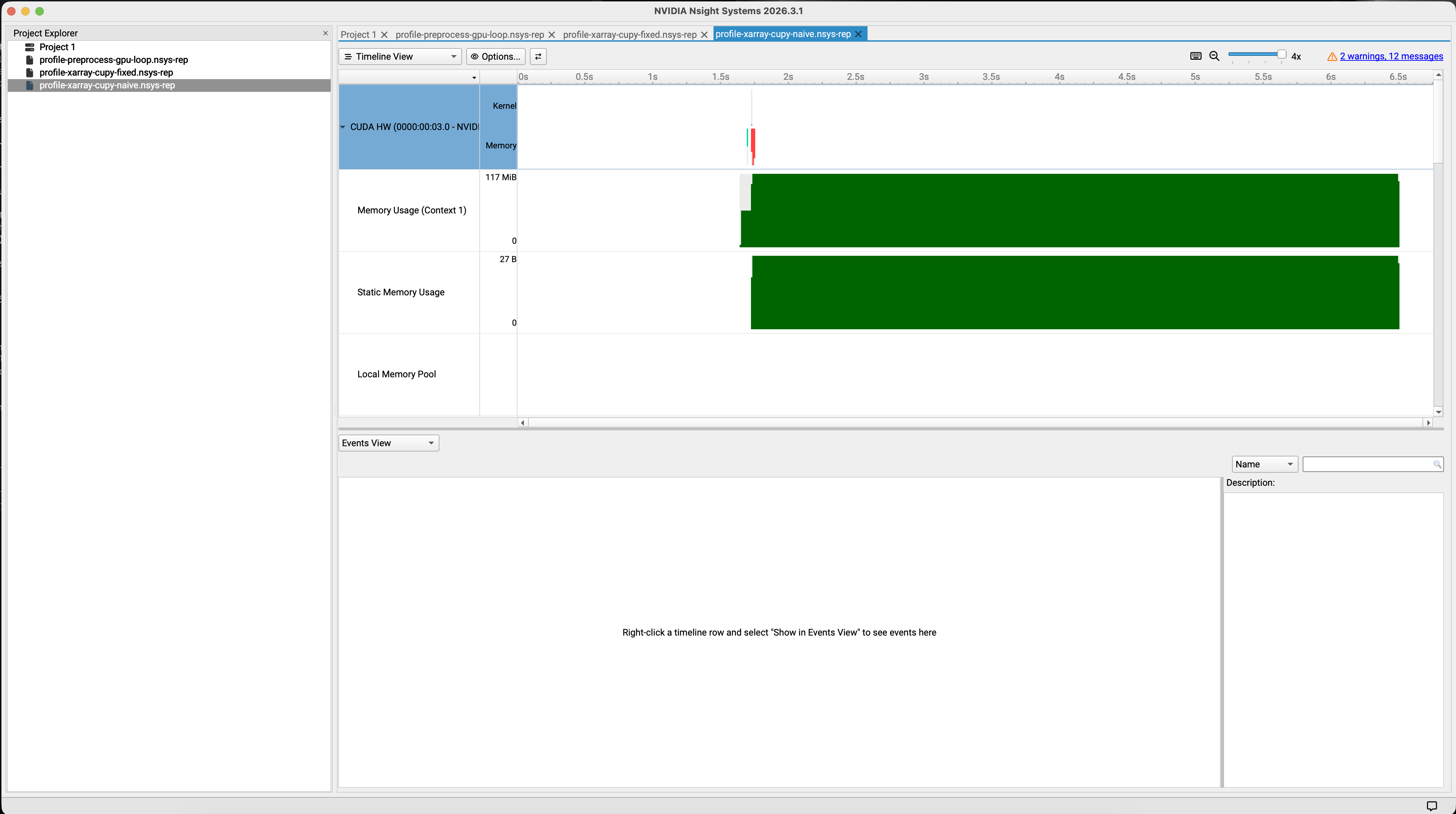
These timelines are dense, so here’s how to read them. Time runs left to right. The rows under CUDA HW show what the GPU actually did: the Kernels row is GPU compute, and the Memory row is the host-to-device and device-to-host copies. When those rows are empty, the GPU is idle. If you are having trouble opening the report, follow the annotated screenshots in this section.
Reading the naive run left to right: a host-to-device cudaMemcpy near the start (the cp.asarray(air) call), a few small kernels for the reshape and mean-subtraction, then a long device-to-host cudaMemcpy (the .get()), and after that a long stretch where the Kernels and Memory rows are empty while the CPU runs SVD. That idle stretch is the bottleneck.
The GPU isn’t absent here. It did some work. The problem is that the expensive operation moved back to the CPU, so the wall-clock time looks a lot like the CPU baseline. This is the common trap: seeing any GPU utilization doesn’t prove the important work ran on the GPU.
Keeping the computation on the GPU
Now keep the SVD on the GPU too. The cleanest way is through cupy-xarray: its .cupy accessor moves the underlying data onto the GPU in place. Once X is a CuPy array, np.linalg.svd dispatches to CuPy’s SVD through NumPy’s __array_function__ protocol, so the same line that ran on the CPU before now runs on the GPU.
The fixed version lives in scripts/xarray-cupy-fixed.py.
The change from the naive version is small but decisive: the .get() round-trip is gone, the data moves onto the GPU through the .cupy accessor, and the SVD now runs on the GPU:
 import xarray as xr
+import cupy_xarray

-air = ds["air"]
-T = cp.asarray(air)
+air = ds["air"].cupy.as_cupy()
+T = air.data

-X = X.get()
 U, S, Vt = np.linalg.svd(X, full_matrices=False)

+cp.cuda.Stream.null.synchronize()
 elapsed = time.perf_counter() - t0
Run it, then capture a timeline:
python scripts/xarray-cupy-fixed.py
nsys profile \
  --trace cuda,osrt \
  --cuda-memory-usage true \
  --force-overwrite true \
  --output profile-xarray-cupy-fixed \
  $(which python) scripts/xarray-cupy-fixed.py
Copy this report down to your laptop and open it in Nsight Systems, the same way you did for the naive run:
brev copy <your-instance-name>:~/profile-xarray-cupy-fixed.nsys-rep .
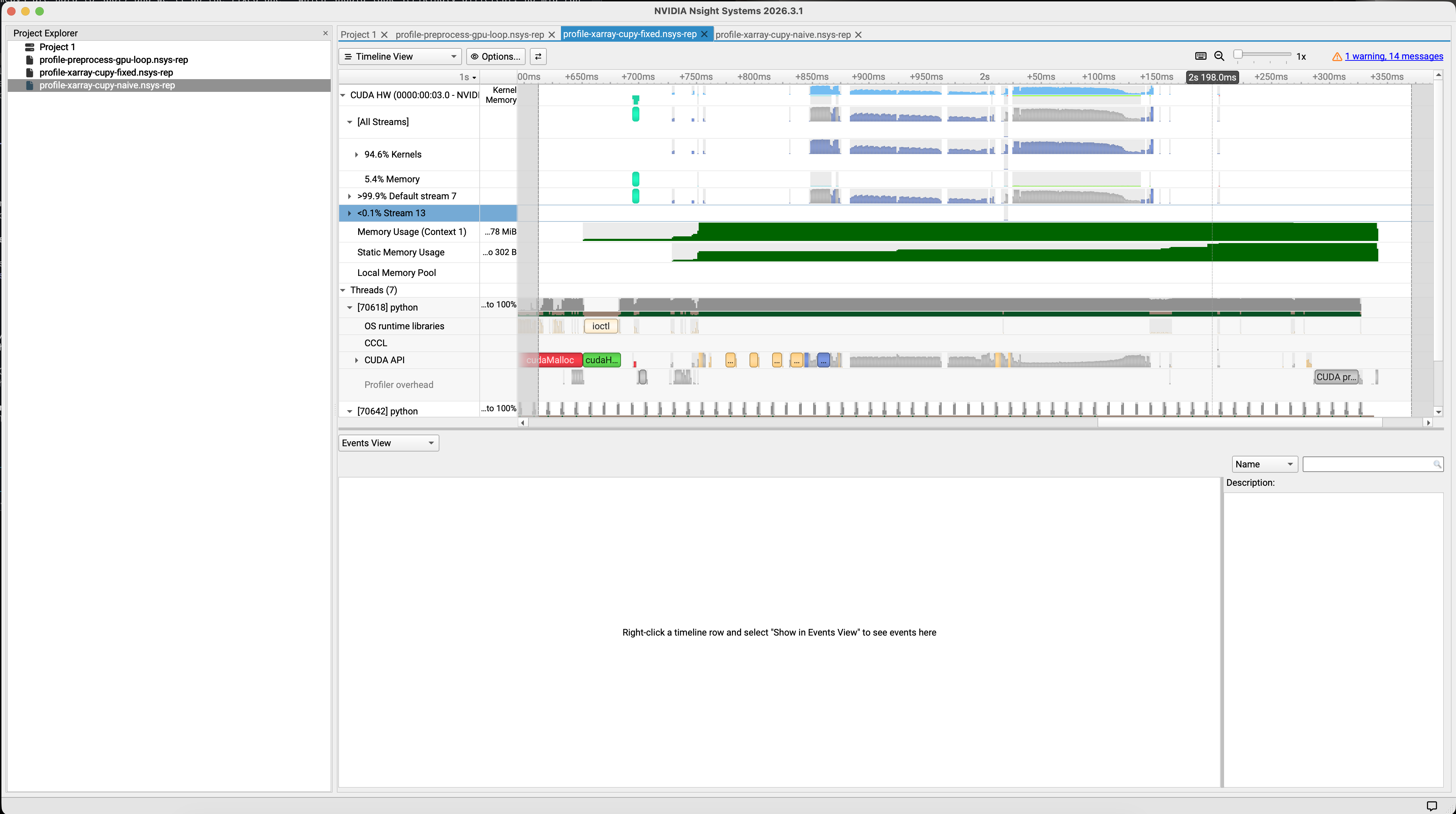
Compared with the naive version, the timeline shows no host-to-device or device-to-host memcpy in the middle of the run, and the long idle stretch is gone. The Kernels row stays busy straight through the SVD. That’s the win.
Run the two versions back to back to compare:
python scripts/xarray-cupy-naive.py
python scripts/xarray-cupy-fixed.py
The CPU baseline and the naive GPU version should land close to each other, because both are bound by the CPU SVD. The fixed version should be several times faster than either. On the L4 we tested this on, that was roughly 5.0s for the CPU baseline, 5.5s for the naive version, and 1.6s for the fixed one, about a 3x speedup. The exact numbers depend on your GPU, so focus on the relationship rather than the seconds. One more check: the first mode variance fraction should match across all three scripts. That’s how you confirm the GPU produced the same answer, not just a faster wrong one.
The fixed version still pays one transfer onto the GPU, but it doesn’t bring the matrix back before the SVD. That’s the real fix. At this size the workload is large enough that running the SVD on the GPU more than pays for the transfer. Once the data is on the GPU, keep the hot path there, and synchronize before timing.
When preprocessing becomes the bottleneck
We fixed the expensive mathematical computation. But a fast SVD doesn’t guarantee a fast program. GPU pipelines usually have a second front: the Python preprocessing that feeds the analysis. A common real step before an EOF analysis is computing per-grid-cell statistics. Here’s the natural, and slow, way to write it.
That non-optimal version lives in scripts/preprocess-cpu-loop.py. Run it and profile it:
python scripts/preprocess-cpu-loop.py
python -m cProfile -o profile-cpu-preprocessing-bad.prof scripts/preprocess-cpu-loop.py
python -m snakeviz -s profile-cpu-preprocessing-bad.prof
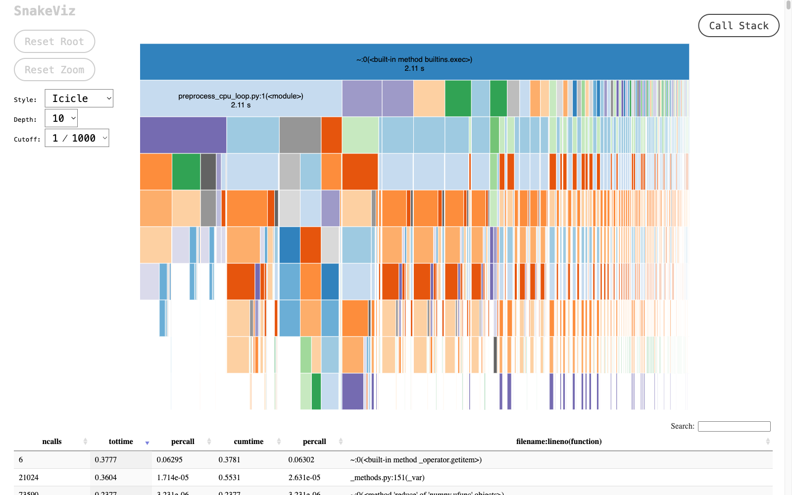
This is where cProfile and SnakeViz shine, and nsys wouldn’t help: there’s no GPU work to put on a timeline. Almost all the runtime sits inside build_features_bad, and the icicle shows why: it fragments into thousands of tiny per-cell numpy calls (mean, std, max/min, var, and the reduce operations beneath them), because each statistic runs once per grid cell across all 10,512 cells.
The tempting fix is to reach for the GPU. But if you keep the per-cell Python loop and just move each cell’s work onto the GPU, you make things worse, not better.
The GPU version lives in scripts/preprocess-gpu-loop.py.
It’s the same per-cell loop as the CPU version, just moved onto the GPU, which is the trap: one tiny kernel launch per cell, thousands of times:
-import numpy as np
+import cupy as cp
 import xarray as xr
+import cupy_xarray

-T = ds["air"].to_numpy()
+T = ds["air"].cupy.as_cupy().data

-def build_features_bad(matrix):
+def build_features_gpu_loop(matrix):
     ncells = matrix.shape[1]
-    features = []
+    features = cp.empty((ncells, 4), dtype=cp.float64)
     for cell in range(ncells):
         column = matrix[:, cell]
-        features.append(
-            (
-                column.mean(),
-                column.std(),
-                column.max() - column.min(),
-                column.var(),
-            )
-        )
-    return np.asarray(features, dtype=np.float64)
+        features[cell, 0] = column.mean()
+        features[cell, 1] = column.std()
+        features[cell, 2] = column.max() - column.min()
+        features[cell, 3] = column.var()
+    cp.cuda.Stream.null.synchronize()
+    return features
Run it once for a clean timing number, then capture a timeline (the nsys run below executes the script again, this time under the profiler):
python scripts/preprocess-gpu-loop.py
nsys profile \
  --trace cuda,osrt \
  --cuda-memory-usage true \
  --force-overwrite true \
  --output profile-preprocess-gpu-loop \
  $(which python) scripts/preprocess-gpu-loop.py
Copy this report down and open it in Nsight Systems as before:
brev copy <your-instance-name>:~/profile-preprocess-gpu-loop.nsys-rep .
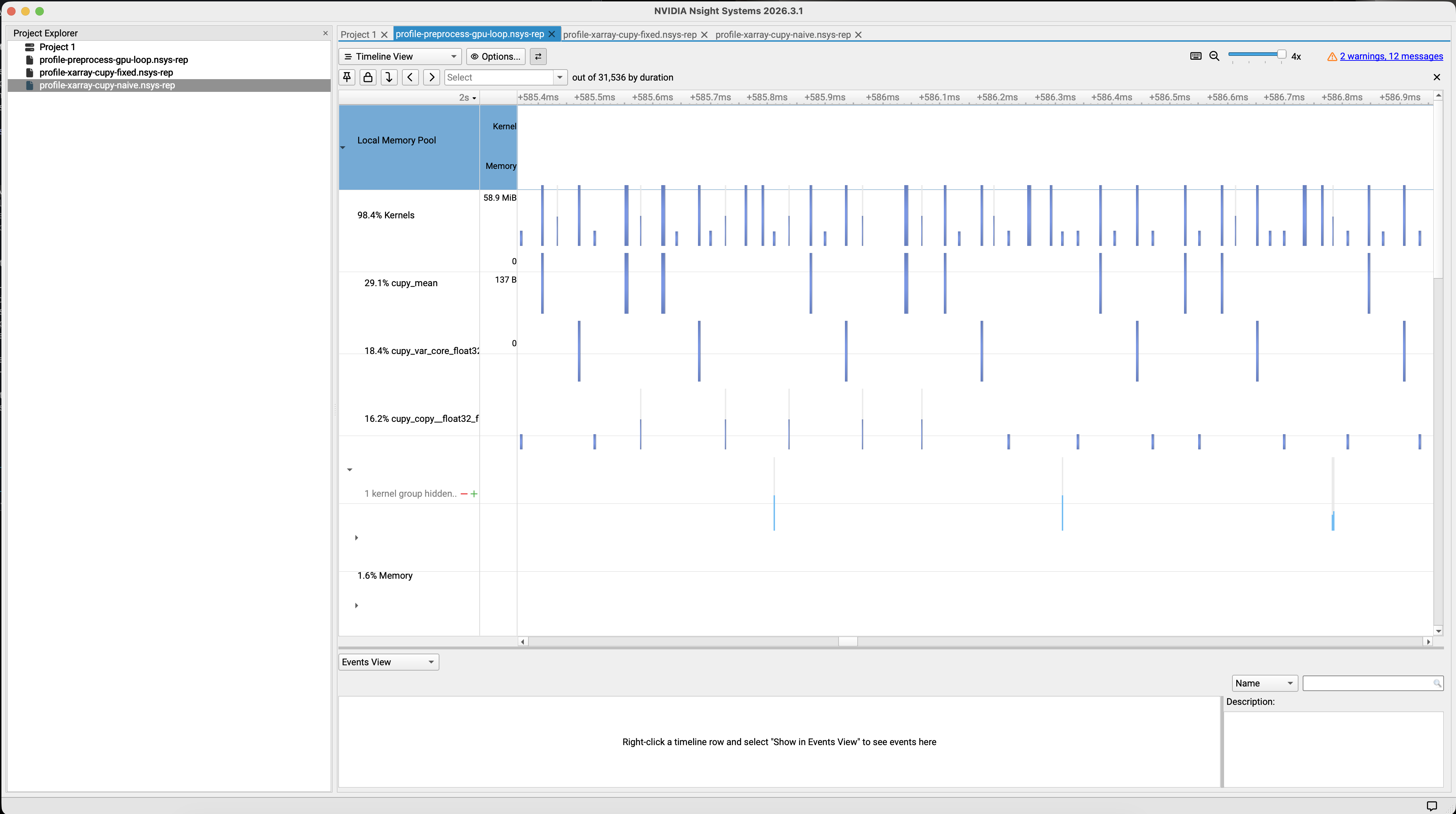
One viewing note for this run: at full zoom it looks like a single solid bar, because there are roughly 150,000 launches packed together. Zoom into a window of a few tens of microseconds and the individual tiny kernels (cupy_mean, cupy_var, and friends) separate out, each followed by a gap. cProfile and SnakeViz would flag the symptom here which is thousands of tiny CuPy calls with a high call count, but they measure Python-side time and can’t show that the GPU sits idle between those launches. The timeline can: a tightly packed row of very short kernel launches with thin gaps between them. Each cell triggers several tiny kernels, and at thousands of cells the launch overhead dominates the actual arithmetic. The GPU spends more time waiting between launches than computing. Using the GPU naively, one tiny operation at a time, is slower than the CPU loop, not faster.
The real fix is to stop looping and let one call process all the cells at once utilizing the strengths of a GPU.
The vectorized version lives in scripts/preprocess-vectorized.py.
The real fix stays on the CPU but replaces the entire per-cell loop with four vectorized calls that run across all cells at once:
-def build_features_bad(matrix):
-    ncells = matrix.shape[1]
-    features = []
-    for cell in range(ncells):
-        column = matrix[:, cell]
-        features.append(
-            (
-                column.mean(),
-                column.std(),
-                column.max() - column.min(),
-                column.var(),
-            )
-        )
-    return np.asarray(features, dtype=np.float64)
+def build_features_fixed(matrix):
+    means = matrix.mean(axis=0)
+    stds = matrix.std(axis=0)
+    ranges = matrix.max(axis=0) - matrix.min(axis=0)
+    variances = matrix.var(axis=0)
+    return np.column_stack((means, stds, ranges, variances))
Run it and compare against the two slow versions:
python scripts/preprocess-cpu-loop.py
python scripts/preprocess-gpu-loop.py
python scripts/preprocess-vectorized.py
The vectorized version replaces thousands of per-cell calls with four calls that run across all cells at once. It should be far faster than both the CPU loop and the GPU loop. On the L4 we tested this on, the CPU loop ran about 0.7s, the per-cell GPU loop about 5s (slower, because of the launch overhead), and the vectorized version about 0.1s. Two lessons come out of this:
- The same vectorized shape is how you’d give the GPU work it likes: fewer, larger operations instead of many tiny ones.
- The vectorized version on the CPU is already fast, so for cheap preprocessing like this you may not need the GPU at all. The honest answer to “should this run on the GPU?” is sometimes no, depending on the size of your workload.
Troubleshooting Nsight Systems
These come up the first time you run nsys on a fresh cloud VM.
On some VMs, the CUDA toolkit wrapper appears first on PATH and reports that Nsight Systems wasn’t installed with that toolkit. If that happens, invoke the system nsys binary directly:
/usr/local/bin/nsys --version
If nsys is found but refuses to run with a permission error, the Nsight Systems directory may be locked down. Make it readable:
sudo chmod 755 /opt/nvidia/nsight-systems
nsys status --environment may also warn that CPU sampling or context-switch tracing is restricted by the kernel. That warning doesn’t block the CUDA timeline examples in this section.
Don’t add --gpu-metrics-devices all unless your VM permits GPU performance counters. On many cloud VMs it fails with an ERR_NVGPUCTRPERM permissions error, and we don’t need GPU metrics for any of the timelines below.
Key Takeaways
The monitoring and profiling tools we covered are useful because they answer different questions:
| Tool | Question it answers |
|---|---|
nvidia-smi |
Does the host see the GPU? |
cuda.core |
Can this Python environment inspect CUDA devices? |
nvtop |
Is a process keeping the GPU busy? |
cProfile + snakeviz |
Is the CPU the real bottleneck? |
nsys |
What do transfers, CPU gaps, synchronization, and kernel launches look like over time? |
And the fixes match the symptoms:
- If data comes back to the CPU before the expensive operation, keep the hot path on the GPU.
- If an inspection or visualization step pulls a full GPU array back to the CPU, reduce, sample, or aggregate on the GPU first.
- If Python preprocessing dominates, vectorize it or move it.
- If many tiny GPU operations dominate, batch them into fewer, larger launches.
- If a task is small and cheap, the CPU may be the right tool. Using the GPU is not always the answer.